Intro

Computational materials researcher specializing in atomistic modeling and data-driven materials
discovery. Experienced in molecular dynamics (MD), density functional theory (DFT), and machine
learning interatomic potentials (MLIP) for property prediction, phase stability, and
mechanism-driven analysis. Expertise in polymerization processes, structure–property relationships,
and ML-integrated simulation workflows for advanced materials design.
Download CV (PDF)
Professional Experience
- Postdoc CNRS | University of Poitiers, Poitiers, France (2025-Present)
- Postdoc Civil Engineering | IIT Delhi, Delhi, India (2025)
- Internship Schrodinger Inc. | Hyderabad, India (2024)
Education
- PhD in Mechanical Engineering | IIT Bombay (2019-2024)
- M.Tech in Nanotechnology | IIT Roorkee (2015-2017)
- B.Tech in Mechanical Engineering | UPTU (2010-2014)
Hobbies & Interests
Contact
Poitiers, France
Work
Workflow to get phonon properties
SNAP potential for Mg2Si(x)Sn(1-x)
Graphene with layers
Graphene with grain boundaries
Graphene with strain, ripples, and curvatures
Thesis
Workflow to get
phonon properties
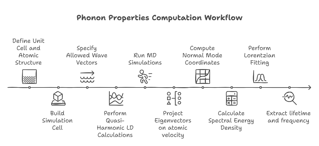
The workflow for computing phonon properties using spectral energy density (SED) analysis begins by
defining the unit cell and atomic structure, which is then used to build the simulation cell.
Allowed wave vectors \( \mathbf{k} \) are specified before performing quasi-harmonic lattice
dynamics (LD) calculations using GULP or Phonopy to obtain wave vectors, frequencies, and mode
shapes (eigenvectors).
Molecular dynamics (MD) simulations are then run in LAMMPS to generate atomic positions and
velocities.
The eigenvectors are projected onto atomic positions and velocities to obtain the normal mode
coordinates \( \mathbf{q} \), which are then used to compute the spectral energy density \( \phi \).
Lorentzian fitting of \( \phi \) extracts the phonon lifetimes \( \tau \) and peak frequencies \(
\omega_0 \), along with thermal conductivity \( \kappa \).
Since the Boltzmann Transport Equation (BTE) requires \( \tau \), this completes the computational
workflow for phonon transport analysis.
SNAP potential for
Mg2Si(x)Sn(1-x)
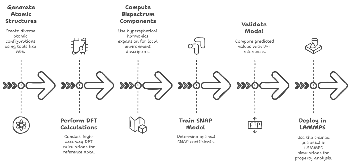
To build a Spectral Neighbor Analysis Potential (SNAP) for a material system like Mg₂Si, one begins
by generating a diverse and representative dataset
of atomic structures that includes not just the pristine bulk phase but also strained
configurations, surfaces, point defects
(such as Mg and Si vacancies or interstitials), thermally perturbed snapshots from ab initio
molecular dynamics, and possibly doped or alloyed
configurations if applicable. These structures are typically created using tools like ASE (Atomic
Simulation Environment), pymatgen, or VESTA,
and must cover a broad configurational space to ensure that the resulting potential can generalize
well. For each of these atomic configurations,
high-accuracy quantum mechanical calculations are performed using Density Functional Theory (DFT)
with packages such as VASP, Quantum ESPRESSO, or GPAW.
The DFT output must include total energies, atomic forces, and stress tensors for every structure.
These serve as the reference data for training the
SNAP model. Next, the bispectrum components that describe each atom's local environment are computed
based on a hyperspherical harmonics expansion,
which encodes geometric information into invariant descriptors. This is done using the FitSNAP
software, a Python-based interface that works with LAMMPS
and is specifically designed for training and applying SNAP potentials. A typical FitSNAP training
input includes definitions for
elements (Mg and Si in this case), the radial cutoff distance (typically ~5.0 Å), the angular
resolution parameter `twojmax` (usually 6–8),
and weighting factors for fitting to energy, force, and stress data. Once the bispectrum features
are generated, a linear least-squares regression
is performed (usually ridge regression with regularization) to determine the optimal SNAP
coefficients that minimize the error between predicted
and DFT reference values. This results in a trained potential file (`snap-model.snap`) and
corresponding parameter file (`snapparam.out`).
The quality of the model is then validated on a test set by comparing predicted vs. DFT energy,
force, and stress values using metrics such as RMSE.
Further validation may involve running LAMMPS simulations (with `pair-style snap`) to compute
material properties like
phonon spectra (via LAMMPS + Phonopy), elastic constants, or thermal conductivity using equilibrium
or non-equilibrium MD. Throughout this process,
the key tools include: structure generation software (ASE, pymatgen), DFT codes (VASP, QE), FitSNAP
for feature computation and training, and LAMMPS
for deployment. Proper data management, hyperparameter tuning (e.g., twojmax, regularization
strength), and cross-validation are critical to ensure
a robust and transferable potential capable of accurately simulating Mg₂Si under various conditions.
Graphene with Layers
Details about phonon transport in multilayer graphene...
Graphene with Grain Boundaries
Exploration of how grain boundaries affect thermal and electronic properties...
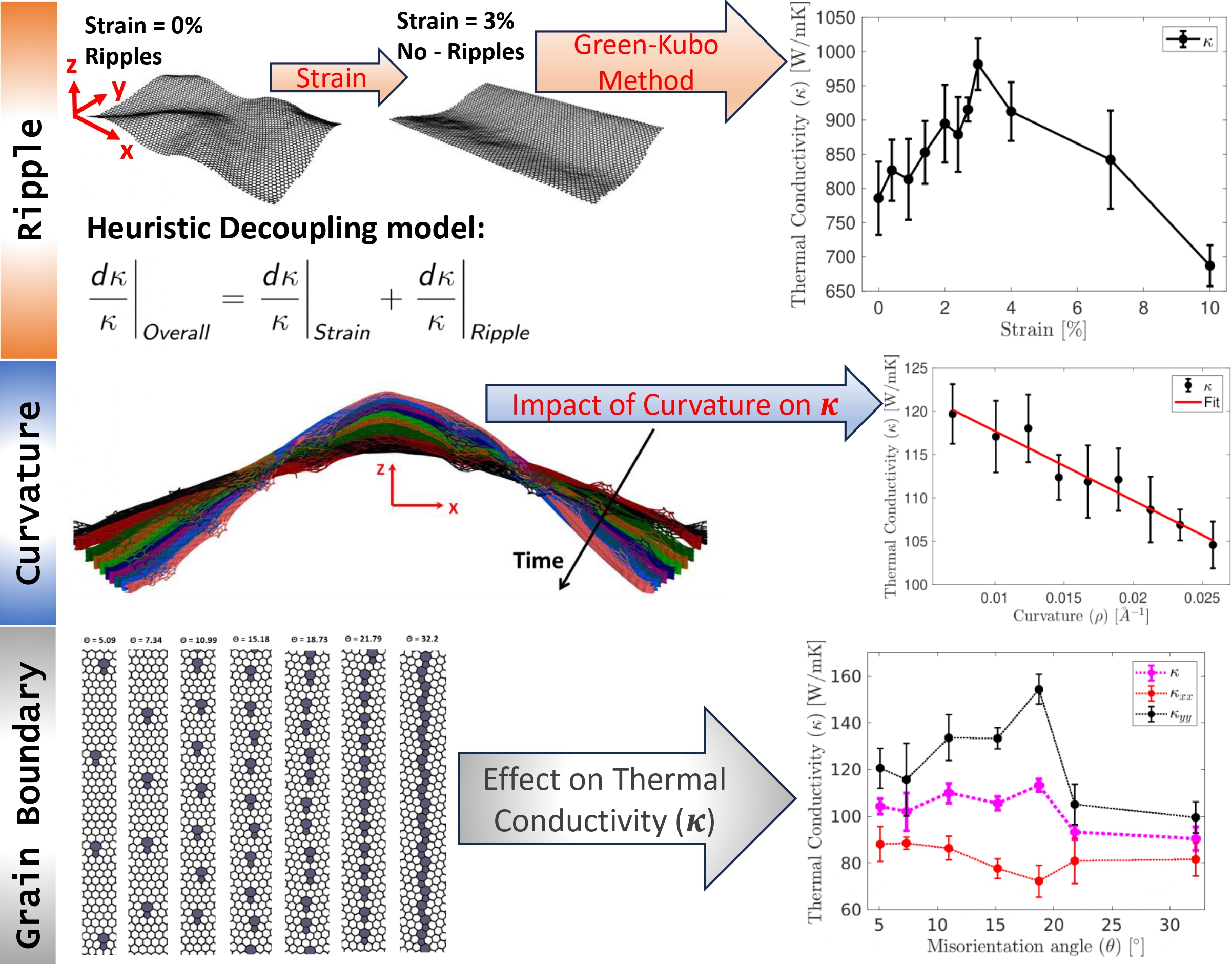
Graphene with Strain, Ripples
and Curvatures
Understanding the impact of mechanical deformations on graphene’s transport properties...
Thesis
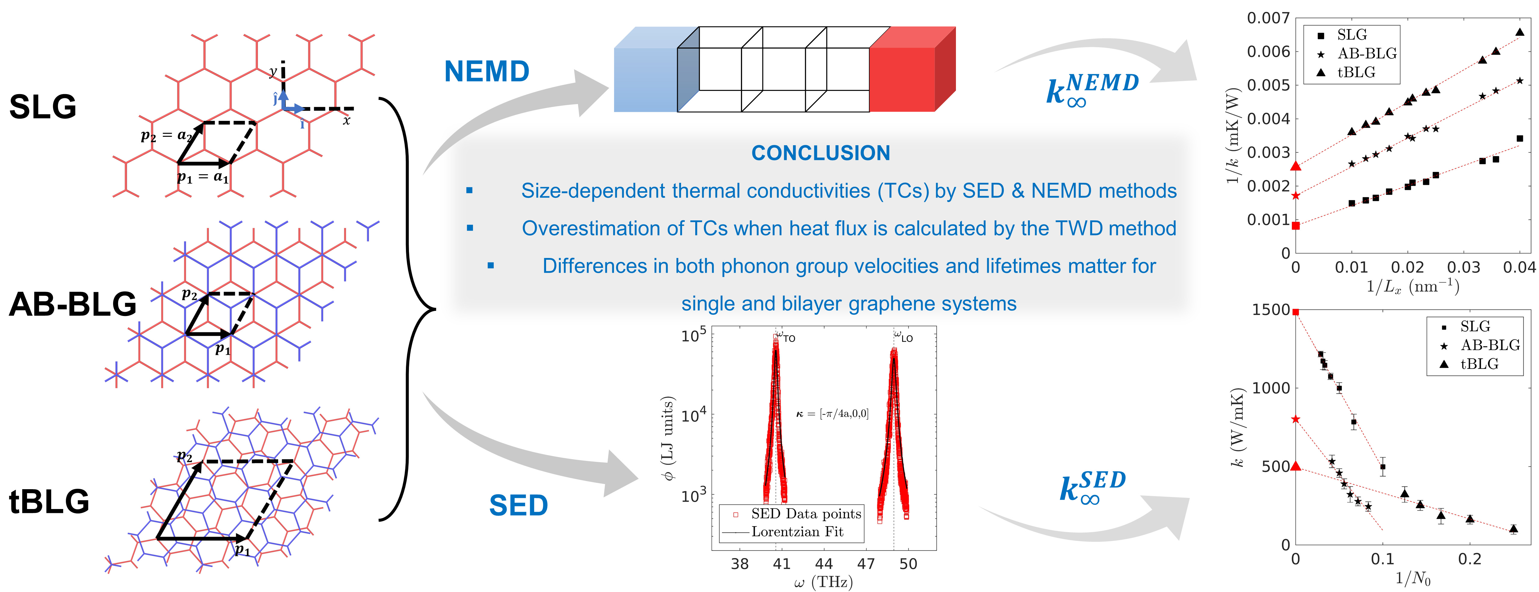
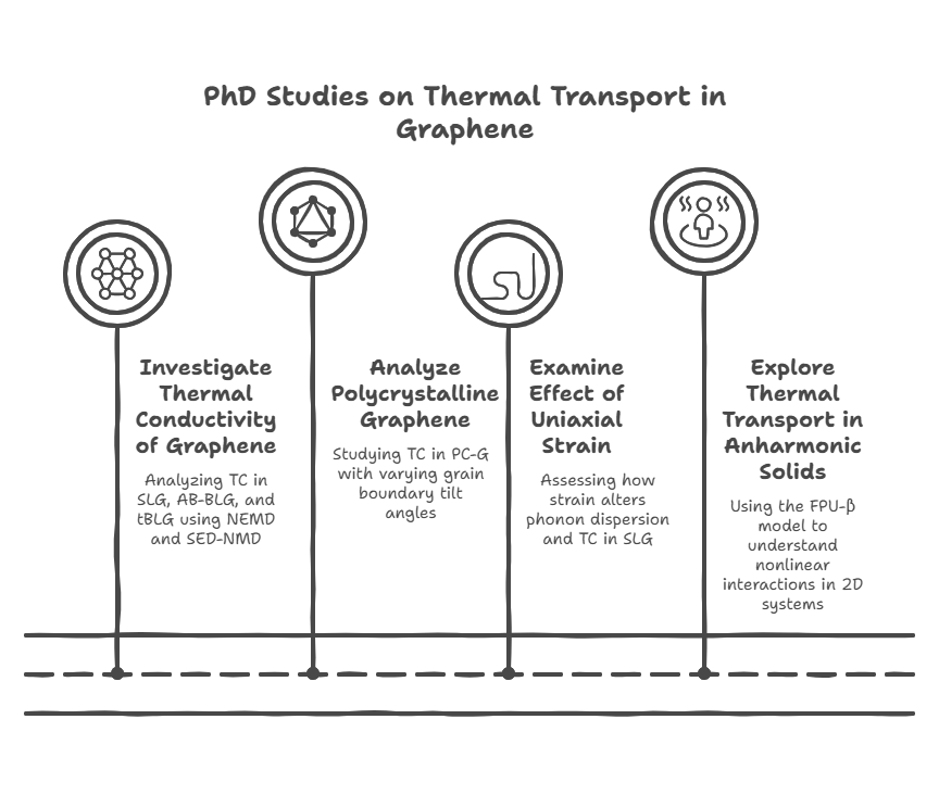
During my PhD, I conducted four key studies to advance the understanding of thermal transport in
graphene and 2D materials. First, I investigated the thermal conductivity (TC) of pristine
single-layer graphene (SLG), AB-stacked bilayer graphene (AB-BLG), and twisted bilayer graphene
(tBLG) using both nonequilibrium molecular dynamics (NEMD) and spectral energy density (SED)-based
normal mode decomposition (NMD), revealing that tBLG exhibits lower phonon group velocities and
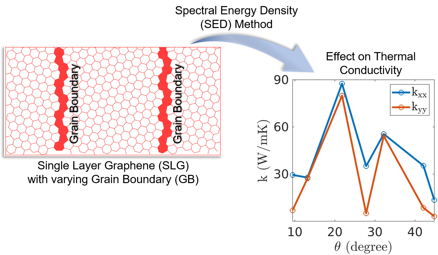
lifetimes, which explains its reduced TC compared to SLG and AB-BLG. Second, I analyzed
polycrystalline graphene (PC-G) with various grain boundary tilt angles, demonstrating that TC
strongly depends on tilt orientation and is not correlated with phonon density of states or average
lifetimes, and I proposed statistical measures to characterize phonon transport based on group
velocity and lifetime distributions. Third, I examined the effect of uniaxial strain on SLG and
found that strain alters the phonon dispersion—especially the ZA mode—causing a shift from quadratic
to linear behavior, and reduces phonon group velocities while leaving lifetimes mostly unchanged,
thereby impacting TC. Finally, I explored thermal transport in 2D anharmonic solids using the
Fermi–Pasta–Ulam (FPU)-β model for the first time, employing both Green-Kubo and NMD methods to
demonstrate the role of nonlinear interactions, with TC showing logarithmic divergence with system
size due to size-dependent phonon lifetimes and velocities. Together, these studies offer deep
insights into phonon behavior and heat conduction mechanisms in both realistic and idealized 2D
systems.
Download
thesis
(PDF)
Blog

Science
How GPU came into picture
### **Chapter: When One Brain Was Not Enough**
There was a time, not too long ago, when every computer in the world relied on a single, powerful
thinker. This thinker was called the CPU, the Central Processing Unit. It was the brain of the
machine, and for decades, engineers believed that if they could just make this brain faster,
everything else would follow.
People like Gordon Moore, working at Intel, observed that computers seemed to double in power every
couple of years. It felt like magic. Every new generation of processors ran faster, handled more
tasks, and made the impossible seem routine. Software grew bolder because hardware kept up.
But nature, as it often does, had its limits.
As engineers pushed CPUs to run faster, the chips began to heat up like overworked engines. Power
consumption soared. The elegant curve of progress began to flatten. It was as if the single thinker
at the center of the computer had reached exhaustion. No matter how much you urged it, it could not
think faster without burning itself out.
And so, the question quietly emerged:
*What if the problem was not how fast one brain could think… but how many brains could think
together?*
---
### **The Artists Who Changed Computing**
While scientists wrestled with slowing CPUs, another world was racing ahead — the world of graphics.
Video games were becoming richer, more detailed, more alive. Companies like NVIDIA and ATI
Technologies were trying to solve a different challenge entirely: how to draw millions of pixels on
a screen, dozens of times every second.
Each pixel was simple. It needed color, light, maybe a shadow. But there were millions of them. And
each one could be computed independently.
This was the crucial realization.
Instead of one powerful thinker, what if you had thousands of small ones, each handling a tiny piece
of the picture?
Thus, the GPU — the Graphics Processing Unit — was born. Not as a rival to the CPU, but as a
specialist. A painter made of many hands.
---
### **A Radical Idea**
At first, GPUs were just artists. They painted images, rendered scenes, and powered games. But deep
inside, something more profound was happening.
The GPU was not just drawing pictures. It was performing the same calculation over and over again,
incredibly fast, across thousands of tiny cores. It was a machine built for repetition, for rhythm,
for parallelism.
And then, in 2006, NVIDIA made a bold move.
They introduced CUDA — the Compute Unified Device Architecture.
With CUDA, they told the world:
*“This machine you thought was just for graphics… can think.”*
Suddenly, scientists, engineers, and programmers could write code that ran directly on the GPU. Not
for images, but for mathematics, physics, and data.
The artist had become a mathematician.
---
### **When Science Discovered Parallel Thinking**
Once the door was opened, entire fields rushed in.
Physicists began simulating atoms and molecules with unprecedented scale. Climate scientists modeled
weather patterns across continents. Biologists folded proteins and studied life at the molecular
level.
All of these problems shared a hidden structure: they could be broken into many small, similar
pieces.
And GPUs were perfect for that.
It was as if, instead of asking one genius to solve a problem, you gathered ten thousand students
and gave each a small part. The answer arrived not through brilliance alone, but through
coordination.
---
### **The Age of Intelligence**
Then came a revolution that changed everything again.
Machine learning.
Researchers like Geoffrey Hinton and teams across the world began building neural networks — systems
inspired by the human brain. These networks required enormous amounts of computation, especially
during training.
At companies like OpenAI, models grew larger and more ambitious. The calculations involved were
staggering — billions upon billions of operations.
The CPU could not keep up.
But the GPU could.
Because deep learning, at its core, is built on matrix multiplication — the very kind of repetitive,
parallel work GPUs were born to do.
Training that once took months could now be done in days. Sometimes hours.
The GPU had found its true calling.
---
### **The Machines Behind the Magic**
Today, a modern GPU like the one you are using — the H100 — is not just a chip. It is a city.
Inside it are thousands of cores working in parallel. Specialized units called Tensor Cores handle
matrix operations with incredible efficiency. High Bandwidth Memory feeds data at breathtaking
speeds.
It is not designed to think like a human.
It is designed to think like a crowd.
---
### **Not Alone in the Race**
Although NVIDIA led this transformation, they were not alone.
AMD built powerful GPUs of their own and developed alternative ecosystems. Intel entered the space
with new architectures, seeking to unify CPU and GPU computing. Google even designed custom chips
called TPUs, tailored specifically for machine learning.
But NVIDIA did something unique.
They did not just build hardware. They built an ecosystem — CUDA, libraries, tools — that made it
easy for developers to stay and build upon their platform.
In technology, this often matters more than raw power.
---
### **The Cost of Power**
Of course, the journey was not without challenges.
GPUs were difficult to program in the beginning. Data movement between CPU and GPU became a
bottleneck. Not every problem could be parallelized. And these machines consumed enormous amounts of
power.
Even today, engineers continue to wrestle with these limitations.
But the direction is clear.
---
### **The Real Lesson**
If you step back from all the details — the chips, the companies, the code — a deeper story emerges.
The rise of the GPU is not just about faster computers.
It is about a shift in how we think about problems.
Once, we believed in the power of a single, ever-faster mind.
Now, we understand the strength of many minds working together.
---
### **A Thought to Carry Forward**
Some problems in life cannot be solved by thinking harder.
They are solved by thinking together.
That is the philosophy embedded in every GPU.
And now, sitting at your machine, running your code, you are not just using a computer.
You are conducting an orchestra of thousands of tiny thinkers, all working in harmony, turning ideas
into reality.
Tools
Programming languages: Python, MATLAB, AWK, C++, Bash, HPC Workflows
Simulation software: VASP, Quantum Espresso, LAMMPS, GULP
MLIP frameworks: MACE, DeepMD, Allegro, Magus, M3GNet, OpenCSP
Structure prediction tools: USPEX, XtalOpt
Visualization and analysis: ASE, Pymatgen, phonopy, vasppy, VESTA, Maestro, Ovito,
VMD
Elements
Text
This is bold and this is strong. This is italic and this is
emphasized.
This is superscript text and this is subscript text.
This is underlined and this is code: for (;;) { ... }. Finally, this is a link.
Heading Level 2
Heading Level 3
Heading Level 4
Heading Level 5
Heading Level 6
Blockquote
Fringilla nisl. Donec accumsan interdum nisi, quis tincidunt felis sagittis eget tempus
euismod. Vestibulum ante ipsum primis in faucibus vestibulum. Blandit adipiscing eu felis
iaculis volutpat ac adipiscing accumsan faucibus. Vestibulum ante ipsum primis in faucibus lorem
ipsum dolor sit amet nullam adipiscing eu felis.
Preformatted
i = 0;

while (!deck.isInOrder()) {
    print 'Iteration ' + i;
    deck.shuffle();
    i++;
}

print 'It took ' + i + ' iterations to sort the deck.';
Lists
Unordered
- Dolor pulvinar etiam.
- Sagittis adipiscing.
- Felis enim feugiat.
Alternate
- Dolor pulvinar etiam.
- Sagittis adipiscing.
- Felis enim feugiat.
Ordered
- Dolor pulvinar etiam.
- Etiam vel felis viverra.
- Felis enim feugiat.
- Dolor pulvinar etiam.
- Etiam vel felis lorem.
- Felis enim et feugiat.
Icons
Actions
Table
Default
| Name |
Description |
Price |
| Item One |
Ante turpis integer aliquet porttitor. |
29.99 |
| Item Two |
Vis ac commodo adipiscing arcu aliquet. |
19.99 |
| Item Three |
Morbi faucibus arcu accumsan lorem. |
29.99 |
| Item Four |
Vitae integer tempus condimentum. |
19.99 |
| Item Five |
Ante turpis integer aliquet porttitor. |
29.99 |
|
100.00 |
Alternate
| Name |
Description |
Price |
| Item One |
Ante turpis integer aliquet porttitor. |
29.99 |
| Item Two |
Vis ac commodo adipiscing arcu aliquet. |
19.99 |
| Item Three |
Morbi faucibus arcu accumsan lorem. |
29.99 |
| Item Four |
Vitae integer tempus condimentum. |
19.99 |
| Item Five |
Ante turpis integer aliquet porttitor. |
29.99 |
|
100.00 |